Forecasting the 2020 US Presidential Election
About the Model:
Much of the political discourse following the 2016 Presidential Election focused on the shortcomings of polling in predicting its outcome. Indeed, every major forecast model (poll-based or otherwise) predicted that Clinton was favored to win, with the Huffington Post and Princeton Election Consortium models predicting a 98% and 99% chance of a Clinton victory, respectively. Such models would have considered Trump’s 304-227 electoral victory a near-impossibility. So where did they go wrong?
Two major problems exist with poll-based models. The first error is a common misinterpretation of polling data - namely, the failure of many pundits and forecasters to realize that polling spreads do not adequately capture the current state of a race. For example, although both of the following theoretical polls have a spread of Clinton +4, a poll with the results (Clinton 52 / Trump 48 / Undecided 0) bodes much better for Clinton than (Clinton 46 / Trump 42 / Undecided 12); in the latter case, if slightly more than 2/3 of the undecideds break for Trump on election day, Trump wins despite Clinton’s ostensible 4-point lead.
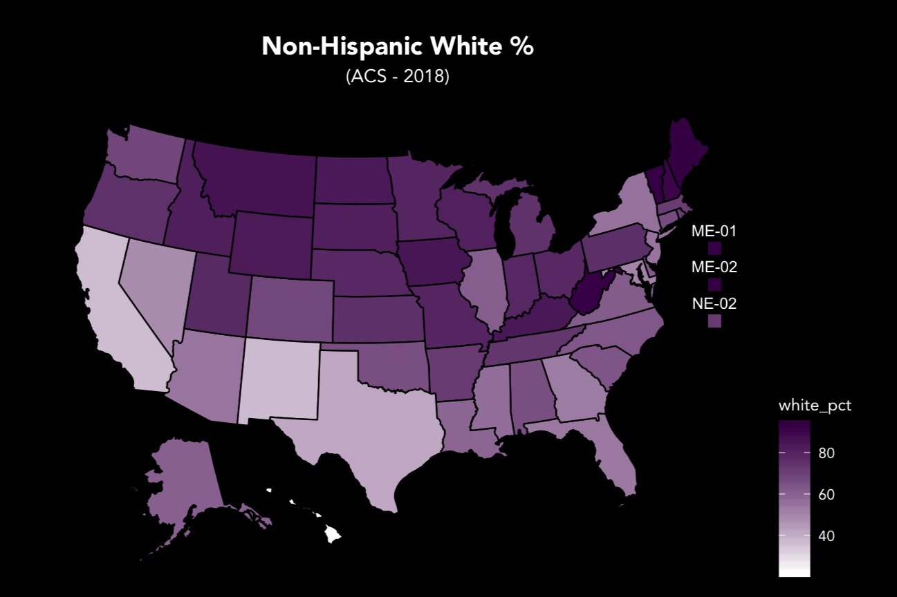
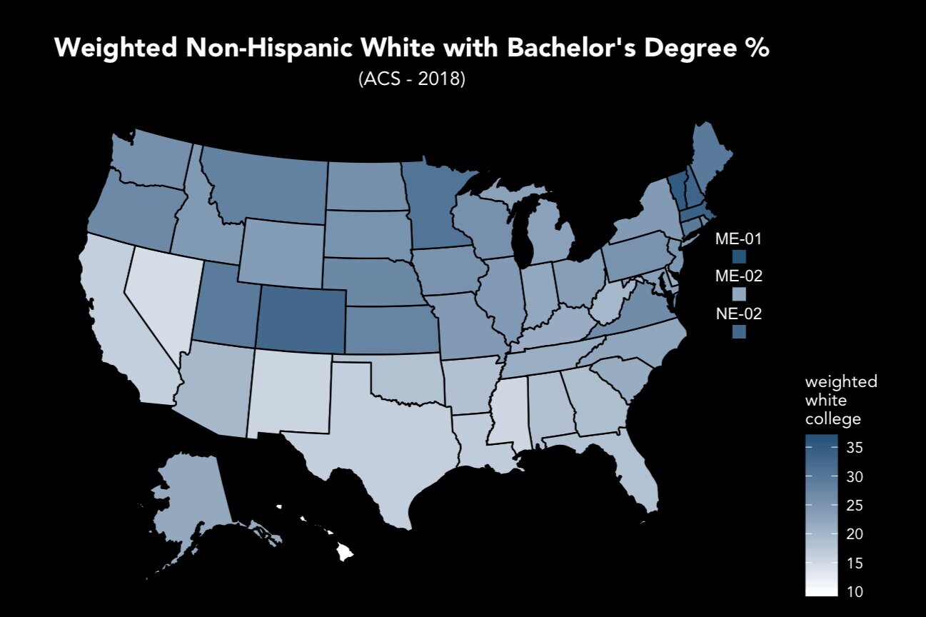
The second problem relates to the methodologies employed by the pollsters themselves - namely, the failure of many state-level polls to adequately weight non-college-educated white voters in their samples. In previous elections, differences in the party preferences of white voters based on educational attainment were minimal; as a result, pollsters’ tendency to oversample college-educated white voters (due to their higher survey completion rate) caused minimal systemic bias.
Pre-2016 realignments saw a drastic increase in the party preference disparity between these two groups; while the 2012 election only showed an 11-point gap, that divide increased to a staggering 35 points in 2016, and remained at 32 points in the 2018 midterms.
Under these new conditions, oversampling of college-educated white voters causes systemic Democratic bias, particularly in states with large populations of white voters without college degrees.

Realignments between 2012 and 2016 drastically increased educational divides in white voters’ party preferences. These shifts appeared to remain for the 2018 midterms.
Data from Pew and the National Election Pool (‘12, ‘16, ‘18) and CNN (‘08).
Wisconsin, Pennsylvania, and Michigan - as the three former “blue wall” states that unexpectedly backed Trump in 2016 and pushed him over 270 - have received an outsized share of attention in post-election analysis. All three have relatively high populations of white voters without college degrees, and consequently, all backed Trump more than polling indicated. However, the narrow focus on these three states led to a flawed conclusion that all polling throughout the country must have underestimated Trump and overestimated Clinton, which is simply not case.
As the map below indicates, while polling in the “rust belt” and midwestern states did in fact overestimate Clinton’s support (in some cases by an extensive margin), polling in the southwestern and west coast states actually consistently underestimated her support. It thus follows that a more-accurate poll-based model cannot simply make a uniform adjustment to the polling in Trump’s favor, but rather must be able to adjust polling margins in both directions.
My model is mostly successful in achieving this, significantly reducing Democratic bias in states like Indiana and Minnesota while also reducing Republican bias in states like Texas and California. While Republican bias increased in the Pacific Northwest and Maine, the overall improvements evinced by the model validation metrics below outweigh these shortcomings. For the 27 states tested, my 2016 electoral college forecast makes 0 misclassifications, with only 7 “tossup” ratings.
Model Validation:


Note: “tossup” ratings are counted as false classifications for recall calculations, excluded for accuracy calculation.
Methods:
Training:
The model was trained on 36 senate and gubernatorial elections from the 2018 midterms for which at least 6 polls were available on RealClearPolitics. National vote intent (Democratic, Republican, and undecided/other) was modeled with a state-space model (SSM) by fitting all “generic congressional ballot” polls between January 1, 2017 and the election using R’s “MARSS” package. Polls were assigned to the median date of the period over which they were conducted; in cases in which multiple polls were assigned the same date, vote intents from each were averaged. Individual states’ polls were regressed against the national fitted values, yielding final state-level intents.
The break from voters in the “undecided” category to the two major parties was modeled using a Bayesian linear model with R’s “rstanarm” package. To prevent overfitting, rstanarm’s “lasso” prior was placed on all coefficients, mimicking frequentist lasso regularization.
Testing:
The model was tested on 27 state and congressional district elections from the 2016 presidential election. National vote intent was modeled using national Clinton vs. Trump polling in the same manner as the training data. State and congressional district polling was also similarly regressed against national intent.
40,000 simulations were conducted, each consisting of the following steps:
Using the fitted SSM state equation for the national polls, a random walk was simulated from November 6th (the last median polling date) to November 8th (the date of the election).
Final state-level vote intents were determined using the adjustments from the previously conducted regressions.
For each state or congressional district, the undecided break was determined with a random draw from the Bayesian model’s posterior distribution.
The final spread for each state or congressional district (with the undecided votes now allocated) was recorded.
Each state’s odds of a Democratic victory was calculated by dividing the number of simulations in which Clinton won by the 40,000 total simulations. Each state was then given a rating based on the victory odds as follows:
0.95 - 1.00 solid dem
0.80 - 0.95 likely dem
0.60 - 0.80 lean dem
0.40 - 0.60 tossup
0.20 - 0.40 lean gop
0.05 - 0.20 likely gop
0.00 - 0.05 solid gop
The Bayesian Model:
A Bayesian approach was selected to better account for uncertainty in each simulation. Rather than a frequentist approach, which would yield a single point prediction for each state’s undecided break, a Bayesian model provides an entire distribution of undecided break predictions, which in turn better informs the final distribution of predicted spreads for each state.

Feature Analysis:


The State-Space Model:
I followed the approach implemented by Orlowski and Stoetzer for modeling multi-party elections, in my case treating the "undecided/other” voters as a single third party. Their approach involves taking natural logs of pairwise combinations of the parties, and provides the distinct advantage of ensuring that all party intents at a given time sum to 100%. For my model, delta represents (democratic intent)/(undecided and other intent) and rho represents (republican intent)/(undecided and other intent).

The final SSM for national polling for the 2016 presidential election.